EBL Photon Density

This notebooko demonstrates the basic use of the EBL photon density class and how to load a model included in the package

[1]:

%matplotlib inline

Imports

[2]:

import matplotlib.pyplot as plt
import numpy as np
from ebltable.ebl_from_model import EBL
import astropy.units as u

[3]:

import astropy.constants as c

Initiate the class plot an example

The easiest way is to import the attenuation from an EBL model. Available models are:

EBL model id	Model ref.	Web link
dominguez	Dominguez et al. (2012)
dominguez-upper	Dominguez et al. (2012)	upper uncertainty bound
dominguez-lower	Dominguez et al. (2012)	lower uncertainty bound
franceschini	Franceschini et al. (2008)	http://www.astro.unipd.it/background/
finke	Finke et al. (2012)	http://www.phy.ohiou.edu/~finke/EBL/
finke2022	Finke et al. (2022)	https://zenodo.org/record/702307
saldana-lopez	Saldana-Lopez et al. (2021)	https://www.ucm.es/blazars/ebl
saldana-lopez-err	Saldana-Lopez et al. (2021) uncertainties	https://www.ucm.es/blazars/ebl
kneiske	Kneiske & Dole (2010)
gilmore	Gilmore et al. (2012)	fiducial model
gilmore-fixed	Gilmore et al. (2012)	fixed model
inoue	Inuoe et al. (2013)	http://www.slac.stanford.edu/~yinoue/Download.html
inoue-low-pop3	Inuoe et al. (2013)	Low pop 3 contribution http://www.slac.stanford.edu/~yinoue/Download.html
inoue-up-pop3	Inuoe et al. (2013)	High pop 3 contribution http://www.slac.stanford.edu/~yinoue/Download.html
cuba	Haardt & Madau (2012)	http://www.ucolick.org/~pmadau/CUBA/HOME.html

[4]:

ebl = {}
for m in EBL.get_models():
    ebl[m] = EBL.readmodel(m)

Define some redshifts and energies for the interpolation:

[5]:

z = np.arange(0.,1.2,0.2)
lmu = np.logspace(-1,3.,100)

Calculate the EBL photon density for all models:

[6]:

nuInu = {}
for m, e in ebl.items():
    nuInu[m] = e.ebl_array(z,lmu)

/Users/manuelmeyer/Python/ebltable/ebltable/interpolate.py:278: RuntimeWarning: Warning: a y value is below interpolation range, y min = 0.00
  warnings.warn(f"Warning: a y value is below interpolation range, y min = {self._y[0]:.2f}",

Do the plot

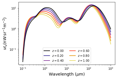
For one EBL model

[7]:

m = 'finke2022'

for i,zz in enumerate(z):
    plt.loglog(lmu,nuInu[m][i],
              ls = '-', color = plt.cm.CMRmap(i / float(len(z))),
               lw = 2.,
              label = '$z = {0:.2f}$'.format(zz),
              zorder= -1 * i)

plt.gca().set_xlabel('Wavelength ($\mu$m)',size = 'x-large')
plt.gca().set_ylabel(r'$\nu I_\nu (\mathrm{nW}\,\mathrm{sr}^{-1}\mathrm{m}^{-2})$',size = 'x-large')
plt.legend(loc = 'lower center', ncol = 2)

[7]:

<matplotlib.legend.Legend at 0x12ec49250>

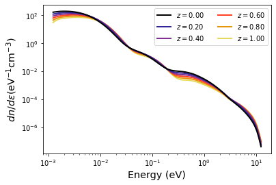
../_images/tutorials_example_ebl_14_1.png

Plot the EBL photon density \(dn / d\epsilon\) instead \(\nu I_\nu\)

convert the wavelength in micrometer to energy in eV:

[8]:

EeV = (c.c.to(u.um / u.s) / (lmu * u.um) * c.h).to(u.eV).value

[9]:

n = ebl[m].n_array(z,EeV)

[10]:

for i,zz in enumerate(z):
    plt.loglog(EeV,n[i],
              ls = '-', color = plt.cm.CMRmap(i / float(len(z))),
               lw = 2.,
              label = '$z = {0:.2f}$'.format(zz),
              zorder= -1 * i)
plt.gca().set_xlabel('Energy (eV)',size = 'x-large')
plt.gca().set_ylabel(r'$dn/d\epsilon (\mathrm{eV}^{-1}\mathrm{cm}^{-3})$',size = 'x-large')
plt.legend(loc = 'upper right', ncol = 2)

[10]:

<matplotlib.legend.Legend at 0x12f37b490>

../_images/tutorials_example_ebl_19_1.png

Print the integrated EBL photon density:

[11]:

ebl[m].ebl_int(0., lmin = 0.01, lmax = 1e3)

[11]:

17.66974687332257

Write the EBL values in a fits file:

[12]:

ebl[m].writefits('out.fits', z, lmu)

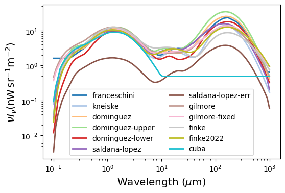
Compare all models

[13]:

plt.figure(dpi=100)

z = 0.

for i,m in enumerate(ebl.keys()):
    plt.loglog(lmu,ebl[m].ebl_array(z, lmu),
              ls = '-',
               color = plt.cm.tab20(i / float(len(ebl.keys()))),
               lw = 2.,
              label = f'{m}')

plt.gca().set_xlabel('Wavelength ($\mu$m)',size = 'x-large')
plt.gca().set_ylabel(r'$\nu I_\nu (\mathrm{nW}\,\mathrm{sr}^{-1}\mathrm{m}^{-2})$',size = 'x-large')
plt.legend(loc = 'lower center', ncol = 2)

/Users/manuelmeyer/Python/ebltable/ebltable/interpolate.py:278: RuntimeWarning: Warning: a y value is below interpolation range, y min = 0.00
  warnings.warn(f"Warning: a y value is below interpolation range, y min = {self._y[0]:.2f}",

[13]:

<matplotlib.legend.Legend at 0x12f82f610>

../_images/tutorials_example_ebl_25_2.png

[ ]: