Optical Depth Interpolation

This notebooko demonstrates the basic use of the optical depth class and how to load a model included in the package

%matplotlib inline

Imports

import matplotlib.pyplot as plt
import numpy as np
from ebltable.tau_from_model import OptDepth

Initiate the class plot an example

The easiest way is to import the attenuation from an EBL model. Available models are:

EBL model id	Model ref.	Web link
dominguez	Dominguez et al. (2012)
dominguez-upper	Dominguez et al. (2012)	upper uncertainty bound
dominguez-lower	Dominguez et al. (2012)	lower uncertainty bound
franceschini	Franceschini et al. (2008)	http://www.astro.unipd.it/background/
finke	Finke et al. (2012)	http://www.phy.ohiou.edu/~finke/EBL/
finke2022	Finke et al. (2022)	https://zenodo.org/record/702307
saldana-lopez	Saldana-Lopez et al. (2021)	https://www.ucm.es/blazars/ebl
saldana-lopez-err	Saldana-Lopez et al. (2021) uncertainties	https://www.ucm.es/blazars/ebl
kneiske	Kneiske & Dole (2010)
gilmore	Gilmore et al. (2012)	fiducial model
gilmore-fixed	Gilmore et al. (2012)	fixed model
inoue	Inuoe et al. (2013)	http://www.slac.stanford.edu/~yinoue/Download.html
inoue-low-pop3	Inuoe et al. (2013)	Low pop 3 contribution http://www.slac.stanford.edu/~yinoue/Download.html
inoue-up-pop3	Inuoe et al. (2013)	High pop 3 contribution http://www.slac.stanford.edu/~yinoue/Download.html

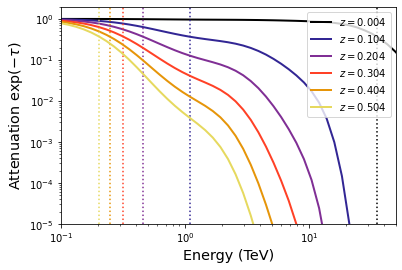
tau =  OptDepth.readmodel(model='finke2022')

Define some redshifts and energies for the interpolation:

z = np.arange(0.004,0.6,0.1)
ETeV = np.logspace(-1,2,50)

For each redshift, calculate the energy where \(\tau = 1\):

Etau1GeV = []
for i,zz in enumerate(z):
    Etau1GeV.append(tau.opt_depth_inverse(zz,1.))

Calculate the attenuation:

atten = np.exp(-1. * tau.opt_depth(z,ETeV))

Do the plot

for i,zz in enumerate(z):
    plt.loglog(ETeV,atten[i],
              ls = '-', color = plt.cm.CMRmap(i / float(len(z))),
              label = '$z = {0:.3f}$'.format(zz), lw = 2)
    plt.axvline(Etau1GeV[i] / 1e3, ls=':', color = plt.cm.CMRmap(i / float(len(z))) )

plt.gca().set_ylim((1e-5,2.))
plt.gca().set_xlim((1e-1,5e1))
plt.gca().set_xlabel('Energy (TeV)',size = 'x-large')
plt.gca().set_ylabel(r'Attenuation $\exp(-\tau)$',size = 'x-large')
plt.legend(loc = 'upper right')

<matplotlib.legend.Legend at 0x12553f760>

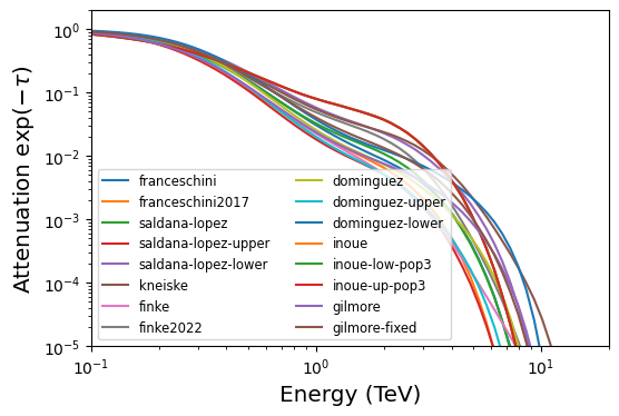
Compare models

tau = {}
for m in OptDepth.get_models():
    tau[m] = OptDepth.readmodel(m)

plt.figure(dpi=100)

ETeV = np.logspace(-2, 1.5,100)
z = 0.3


for m, t in tau.items():
    plt.loglog(ETeV, np.exp(-t.opt_depth(z, ETeV)), label=f"{m}")

plt.gca().set_ylim((1e-5,2.))
plt.gca().set_xlim((1e-1,2e1))
plt.gca().set_xlabel('Energy (TeV)',size = 'x-large')
plt.gca().set_ylabel(r'Attenuation $\exp(-\tau)$',size = 'x-large')
plt.legend(loc='lower left', ncol=2, fontsize='small')

<matplotlib.legend.Legend at 0x1260ef880>